{
  "id": 171810,
  "title": "Lightweight siamese network solution (ResNet18 -> PB 0.8966)",
  "url": "/competitions/prostate-cancer-grade-assessment/discussion/171810",
  "author_name": "Giovanni Cavallin",
  "post_date": "2020-08-02T15:08:04.505000",
  "votes": 4,
  "comment_count": 0,
  "views": 0,
  "content": "<p>In this post I present the ideas for the <a href=\"https://www.kaggle.com/c/prostate-cancer-grade-assessment/overview\">PANDA</a> Kaggle competition.\nPlease refer to the description of the competition for more insights.\n<a href=\"https://github.com/chiamonni/\">@chiamonni</a> and <a href=\"https://github.com/mawanda-jun/\"></a><a href=\"/mawanda\">@mawanda</a>-jun worked on this project (<a href=\"https://github.com/chiamonni/PANDA_Kaggle_competition\">repo</a>).</p>\n\n<h1>Contents</h1>\n\n<ul>\n<li>Problem overview</li>\n<li>Dataset approach</li>\n<li>Network architecture</li>\n<li>Results</li>\n</ul>\n\n<h1>Problem overview</h1>\n\n<p>The Prostate cANcer graDe Assessment (PANDA) Challenge requires participants to recognize 5 severity levels of prostate cancer in prostate biopsy, plus its absence (6 classes).</p>\n\n<p><img src=\"https://storage.googleapis.com/kaggle-media/competitions/PANDA/Screen%20Shot%202020-04-08%20at%202.03.53%20PM.png\" alt=\"Illustration of the biopsy grading assigment\"></p>\n\n<p>Therefore, this is a classification task.</p>\n\n<p>The main challenges Kagglers faced where related to:\n- <strong>dimensionality</strong>: images were quite large and sparse (~50K x ~50K px);\n- <strong>uncertainty</strong>: labels were given by experts, which were sometimes interpreting the cancer gravity in different ways.</p>\n\n<p><img src=\"https://www.googleapis.com/download/storage/v1/b/kaggle-user-content/o/inbox%2F2101276%2Ffe60ff9e1ab7555ba3c4f3f1866631b2%2F192863a82b5a954ba0fa56b910574e1a.jpeg?generation=1596380531799397&amp;alt=media\" alt=\"cancer image\"></p>\n\n<h1>Dataset approach</h1>\n\n<p>I decided to analyze each image and extract relevant \"crops\" to be stored directly on disk in order to reduce compute time while reading the images from disk.\nTherefore, I used the 4x reduced images (level 1 of original dataset) and extracted squared patches of 256px with the \"akensert\" <a href=\"https://www.kaggle.com/akensert/panda-optimized-tiling-tf-data-dataset\">method</a>.\nThen, I stored the crops in an image with the slideshow of crops.</p>\n\n<p><img src=\"https://www.googleapis.com/download/storage/v1/b/kaggle-user-content/o/inbox%2F2101276%2Fcc3ab4fed6daa78c122b54d8a80a9d31%2F0b6e34bf65ee0810c1a4bf702b667c88.jpeg?generation=1596380612573127&amp;alt=media\" alt=\"akensert crops\"></p>\n\n<p>Each image came with a different number of crops.\nSo, I realized a binned graph counting how many times a certain number of crops occured.\nThe \"akensert\" method is the first metioned, the \"cropped\" one is a simple \"strided\" crop, in which I kept each square that was at least covered with 20% of non-zero pixels.</p>\n\n<p><img src=\"https://www.googleapis.com/download/storage/v1/b/kaggle-user-content/o/inbox%2F2101276%2F1aee3408042bed534ee52feb5148860a%2Fnumber_crops_personal_akensert.png?generation=1596380665002903&amp;alt=media\" alt=\"number of crops\"></p>\n\n<p>From the graph it is clear that the \"akensert\" method is more reliable (the curve is tighter) than the first I explored.\nIn addition, I decided to select 26 random selected crops from each image:\n- in the case they were less than 13 I doubled them, and filled the remaining with empty squares;\n- in the case they were more, I randomly selected 26. I thought about this method as a regularization. In fact, the labels could have been assigned wrongly and selecting only a part of the crops could lead to a better generalization capability of my model.\nIn addition, I forced my model to understand the gravity of the cancer from a part of the whole image in the 40% of the dataset, which I think helped it to generalize the proble better.</p>\n\n<h2>Dataset augmentation</h2>\n\n<p>I found out that modifying the color of the images (with random contrast/saturation/ecc) augmentations was not giving me any particular advantage.\nIn addition, I found out that simple flipping/rotation really helped me out in leveraging the differences between CV and LB.\nI also added a random occlusion augmentation, which covered each crop with a rectangle of ranging size of [0, 224) and really helped me in generalize the model performance w.r.t. the LB.\nAs a side note, I think that those augmentations really helped my model perform so well in the private leader board (I gained +3% accuracy).</p>\n\n<p><img src=\"https://www.googleapis.com/download/storage/v1/b/kaggle-user-content/o/inbox%2F2101276%2Fe3889ccbe4626e95b3a1bc5eeabf6946%2Ftest.jpeg?generation=1596380705355303&amp;alt=media\" alt=\"test\"></p>\n\n<p>An example of the resulting augmentations, with 8x8 crops.</p>\n\n<h1>Network architecture</h1>\n\n<p>For the network architecture I took inspiration from the method used from experts, that is:\n1. look closely to the tissue;\n2. characterize each tissue part with the most present gravity of cancer patterns;\n3. take the two most present ones and declare the cancer class.</p>\n\n<p>Therefore, I created a siamese network which received each crop at a time with shared weights. \nThe output of each siamese branch was then <strong>averaged</strong> with the others as a sort of polling, and then brought to the <a href=\"https://www.kaggle.com/haqishen/train-efficientnet-b0-w-36-tiles-256-lb0-87\">binned</a> output.\nSee the image below for further insight.</p>\n\n<p><img src=\"https://www.googleapis.com/download/storage/v1/b/kaggle-user-content/o/inbox%2F2101276%2Fc96851ac147d872029fa0cd09de4daab%2Fnetwork_architecture.png?generation=1596380747042850&amp;alt=media\" alt=\"network architecture\"></p>\n\n<p>Since my computing resources were limited in memory (8GB VRAM, Nvidia 2070s) I was able to train this network with a <a href=\"https://github.com/facebookresearch/semi-supervised-ImageNet1K-models\">ResNet18 semi-weakly pretrained</a> model.</p>\n\n<h1>Cross-validation</h1>\n\n<p>Since my model was performing so coherently among the CV and LB I decided not to do any cross validation. \nIn fact, I simply trained the model with a 70/30 train/validation split of the whole training set.</p>\n\n<h1>Hyper parameters selection</h1>\n\n<p>The best hyper parameters I selected, within the trained weights, are under the folder <code>good_experiments</code>.</p>\n\n<h1>Results</h1>\n\n<p>The aforementioned architecture resulted in:\n- CV: 0.8504\n- LB: 0.8503\n- PB: 0.8966</p>\n\n<p>Those results are quite interesting, since most of the competition participant used a EfficientNetB0 which is far bigger and more accurate in most benchmarks.\nI would have liked to train this particular architecture on a bigger machine, with more interesting architectures, hopefully with even better results.</p>",
  "messages": [
    {
      "id": 955341,
      "postDate": "2020-08-02T15:08:04.507Z",
      "content": "<p>In this post I present the ideas for the <a href=\"https://www.kaggle.com/c/prostate-cancer-grade-assessment/overview\">PANDA</a> Kaggle competition.\nPlease refer to the description of the competition for more insights.\n<a href=\"https://github.com/chiamonni/\">@chiamonni</a> and <a href=\"https://github.com/mawanda-jun/\"></a><a href=\"/mawanda\">@mawanda</a>-jun worked on this project (<a href=\"https://github.com/chiamonni/PANDA_Kaggle_competition\">repo</a>).</p>\n\n<h1>Contents</h1>\n\n<ul>\n<li>Problem overview</li>\n<li>Dataset approach</li>\n<li>Network architecture</li>\n<li>Results</li>\n</ul>\n\n<h1>Problem overview</h1>\n\n<p>The Prostate cANcer graDe Assessment (PANDA) Challenge requires participants to recognize 5 severity levels of prostate cancer in prostate biopsy, plus its absence (6 classes).</p>\n\n<p><img src=\"https://storage.googleapis.com/kaggle-media/competitions/PANDA/Screen%20Shot%202020-04-08%20at%202.03.53%20PM.png\" alt=\"Illustration of the biopsy grading assigment\"></p>\n\n<p>Therefore, this is a classification task.</p>\n\n<p>The main challenges Kagglers faced where related to:\n- <strong>dimensionality</strong>: images were quite large and sparse (~50K x ~50K px);\n- <strong>uncertainty</strong>: labels were given by experts, which were sometimes interpreting the cancer gravity in different ways.</p>\n\n<p><img src=\"https://www.googleapis.com/download/storage/v1/b/kaggle-user-content/o/inbox%2F2101276%2Ffe60ff9e1ab7555ba3c4f3f1866631b2%2F192863a82b5a954ba0fa56b910574e1a.jpeg?generation=1596380531799397&amp;alt=media\" alt=\"cancer image\"></p>\n\n<h1>Dataset approach</h1>\n\n<p>I decided to analyze each image and extract relevant \"crops\" to be stored directly on disk in order to reduce compute time while reading the images from disk.\nTherefore, I used the 4x reduced images (level 1 of original dataset) and extracted squared patches of 256px with the \"akensert\" <a href=\"https://www.kaggle.com/akensert/panda-optimized-tiling-tf-data-dataset\">method</a>.\nThen, I stored the crops in an image with the slideshow of crops.</p>\n\n<p><img src=\"https://www.googleapis.com/download/storage/v1/b/kaggle-user-content/o/inbox%2F2101276%2Fcc3ab4fed6daa78c122b54d8a80a9d31%2F0b6e34bf65ee0810c1a4bf702b667c88.jpeg?generation=1596380612573127&amp;alt=media\" alt=\"akensert crops\"></p>\n\n<p>Each image came with a different number of crops.\nSo, I realized a binned graph counting how many times a certain number of crops occured.\nThe \"akensert\" method is the first metioned, the \"cropped\" one is a simple \"strided\" crop, in which I kept each square that was at least covered with 20% of non-zero pixels.</p>\n\n<p><img src=\"https://www.googleapis.com/download/storage/v1/b/kaggle-user-content/o/inbox%2F2101276%2F1aee3408042bed534ee52feb5148860a%2Fnumber_crops_personal_akensert.png?generation=1596380665002903&amp;alt=media\" alt=\"number of crops\"></p>\n\n<p>From the graph it is clear that the \"akensert\" method is more reliable (the curve is tighter) than the first I explored.\nIn addition, I decided to select 26 random selected crops from each image:\n- in the case they were less than 13 I doubled them, and filled the remaining with empty squares;\n- in the case they were more, I randomly selected 26. I thought about this method as a regularization. In fact, the labels could have been assigned wrongly and selecting only a part of the crops could lead to a better generalization capability of my model.\nIn addition, I forced my model to understand the gravity of the cancer from a part of the whole image in the 40% of the dataset, which I think helped it to generalize the proble better.</p>\n\n<h2>Dataset augmentation</h2>\n\n<p>I found out that modifying the color of the images (with random contrast/saturation/ecc) augmentations was not giving me any particular advantage.\nIn addition, I found out that simple flipping/rotation really helped me out in leveraging the differences between CV and LB.\nI also added a random occlusion augmentation, which covered each crop with a rectangle of ranging size of [0, 224) and really helped me in generalize the model performance w.r.t. the LB.\nAs a side note, I think that those augmentations really helped my model perform so well in the private leader board (I gained +3% accuracy).</p>\n\n<p><img src=\"https://www.googleapis.com/download/storage/v1/b/kaggle-user-content/o/inbox%2F2101276%2Fe3889ccbe4626e95b3a1bc5eeabf6946%2Ftest.jpeg?generation=1596380705355303&amp;alt=media\" alt=\"test\"></p>\n\n<p>An example of the resulting augmentations, with 8x8 crops.</p>\n\n<h1>Network architecture</h1>\n\n<p>For the network architecture I took inspiration from the method used from experts, that is:\n1. look closely to the tissue;\n2. characterize each tissue part with the most present gravity of cancer patterns;\n3. take the two most present ones and declare the cancer class.</p>\n\n<p>Therefore, I created a siamese network which received each crop at a time with shared weights. \nThe output of each siamese branch was then <strong>averaged</strong> with the others as a sort of polling, and then brought to the <a href=\"https://www.kaggle.com/haqishen/train-efficientnet-b0-w-36-tiles-256-lb0-87\">binned</a> output.\nSee the image below for further insight.</p>\n\n<p><img src=\"https://www.googleapis.com/download/storage/v1/b/kaggle-user-content/o/inbox%2F2101276%2Fc96851ac147d872029fa0cd09de4daab%2Fnetwork_architecture.png?generation=1596380747042850&amp;alt=media\" alt=\"network architecture\"></p>\n\n<p>Since my computing resources were limited in memory (8GB VRAM, Nvidia 2070s) I was able to train this network with a <a href=\"https://github.com/facebookresearch/semi-supervised-ImageNet1K-models\">ResNet18 semi-weakly pretrained</a> model.</p>\n\n<h1>Cross-validation</h1>\n\n<p>Since my model was performing so coherently among the CV and LB I decided not to do any cross validation. \nIn fact, I simply trained the model with a 70/30 train/validation split of the whole training set.</p>\n\n<h1>Hyper parameters selection</h1>\n\n<p>The best hyper parameters I selected, within the trained weights, are under the folder <code>good_experiments</code>.</p>\n\n<h1>Results</h1>\n\n<p>The aforementioned architecture resulted in:\n- CV: 0.8504\n- LB: 0.8503\n- PB: 0.8966</p>\n\n<p>Those results are quite interesting, since most of the competition participant used a EfficientNetB0 which is far bigger and more accurate in most benchmarks.\nI would have liked to train this particular architecture on a bigger machine, with more interesting architectures, hopefully with even better results.</p>",
      "rawMarkdown": "In this post I present the ideas for the [PANDA](https://www.kaggle.com/c/prostate-cancer-grade-assessment/overview) Kaggle competition.\nPlease refer to the description of the competition for more insights.\n[@chiamonni](https://github.com/chiamonni/) and [@mawanda-jun](https://github.com/mawanda-jun/) worked on this project ([repo](https://github.com/chiamonni/PANDA_Kaggle_competition)).\n\n# Contents\n- [Problem overview](#problem-overview)\n- [Dataset approach](#dataset-approach)\n- [Network architecture](#network-architecture)\n- [Results](#results)\n\n\n# Problem overview\nThe Prostate cANcer graDe Assessment (PANDA) Challenge requires participants to recognize 5 severity levels of prostate cancer in prostate biopsy, plus its absence (6 classes).\n\n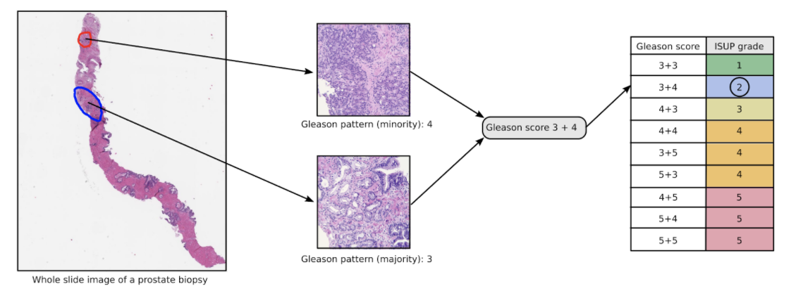![Illustration of the biopsy grading assigment](https://storage.googleapis.com/kaggle-media/competitions/PANDA/Screen%20Shot%202020-04-08%20at%202.03.53%20PM.png)\n\nTherefore, this is a classification task.\n\nThe main challenges Kagglers faced where related to:\n- **dimensionality**: images were quite large and sparse (~50K x ~50K px);\n- **uncertainty**: labels were given by experts, which were sometimes interpreting the cancer gravity in different ways.\n\n![cancer image](https://www.googleapis.com/download/storage/v1/b/kaggle-user-content/o/inbox%2F2101276%2Ffe60ff9e1ab7555ba3c4f3f1866631b2%2F192863a82b5a954ba0fa56b910574e1a.jpeg?generation=1596380531799397&amp;alt=media)\n\n\n# Dataset approach\nI decided to analyze each image and extract relevant \"crops\" to be stored directly on disk in order to reduce compute time while reading the images from disk.\nTherefore, I used the 4x reduced images (level 1 of original dataset) and extracted squared patches of 256px with the \"akensert\" [method](https://www.kaggle.com/akensert/panda-optimized-tiling-tf-data-dataset).\nThen, I stored the crops in an image with the slideshow of crops.\n\n![akensert crops](https://www.googleapis.com/download/storage/v1/b/kaggle-user-content/o/inbox%2F2101276%2Fcc3ab4fed6daa78c122b54d8a80a9d31%2F0b6e34bf65ee0810c1a4bf702b667c88.jpeg?generation=1596380612573127&amp;alt=media)\n\n\nEach image came with a different number of crops.\nSo, I realized a binned graph counting how many times a certain number of crops occured.\nThe \"akensert\" method is the first metioned, the \"cropped\" one is a simple \"strided\" crop, in which I kept each square that was at least covered with 20% of non-zero pixels.\n\n![number of crops](https://www.googleapis.com/download/storage/v1/b/kaggle-user-content/o/inbox%2F2101276%2F1aee3408042bed534ee52feb5148860a%2Fnumber_crops_personal_akensert.png?generation=1596380665002903&amp;alt=media)\n\n\nFrom the graph it is clear that the \"akensert\" method is more reliable (the curve is tighter) than the first I explored.\nIn addition, I decided to select 26 random selected crops from each image:\n- in the case they were less than 13 I doubled them, and filled the remaining with empty squares;\n- in the case they were more, I randomly selected 26. I thought about this method as a regularization. In fact, the labels could have been assigned wrongly and selecting only a part of the crops could lead to a better generalization capability of my model.\nIn addition, I forced my model to understand the gravity of the cancer from a part of the whole image in the 40% of the dataset, which I think helped it to generalize the proble better.\n\n## Dataset augmentation\nI found out that modifying the color of the images (with random contrast/saturation/ecc) augmentations was not giving me any particular advantage.\nIn addition, I found out that simple flipping/rotation really helped me out in leveraging the differences between CV and LB.\nI also added a random occlusion augmentation, which covered each crop with a rectangle of ranging size of [0, 224) and really helped me in generalize the model performance w.r.t. the LB.\nAs a side note, I think that those augmentations really helped my model perform so well in the private leader board (I gained +3% accuracy).\n\n![test](https://www.googleapis.com/download/storage/v1/b/kaggle-user-content/o/inbox%2F2101276%2Fe3889ccbe4626e95b3a1bc5eeabf6946%2Ftest.jpeg?generation=1596380705355303&amp;alt=media)\n\nAn example of the resulting augmentations, with 8x8 crops.\n\n# Network architecture\nFor the network architecture I took inspiration from the method used from experts, that is:\n1. look closely to the tissue;\n2. characterize each tissue part with the most present gravity of cancer patterns;\n3. take the two most present ones and declare the cancer class.\n\nTherefore, I created a siamese network which received each crop at a time with shared weights. \nThe output of each siamese branch was then **averaged** with the others as a sort of polling, and then brought to the [binned](https://www.kaggle.com/haqishen/train-efficientnet-b0-w-36-tiles-256-lb0-87) output.\nSee the image below for further insight.\n\n![network architecture](https://www.googleapis.com/download/storage/v1/b/kaggle-user-content/o/inbox%2F2101276%2Fc96851ac147d872029fa0cd09de4daab%2Fnetwork_architecture.png?generation=1596380747042850&amp;alt=media)\n\nSince my computing resources were limited in memory (8GB VRAM, Nvidia 2070s) I was able to train this network with a [ResNet18 semi-weakly pretrained](https://github.com/facebookresearch/semi-supervised-ImageNet1K-models) model.\n\n# Cross-validation\nSince my model was performing so coherently among the CV and LB I decided not to do any cross validation. \nIn fact, I simply trained the model with a 70/30 train/validation split of the whole training set.\n\n# Hyper parameters selection\nThe best hyper parameters I selected, within the trained weights, are under the folder `good_experiments`.\n\n# Results\nThe aforementioned architecture resulted in:\n- CV: 0.8504\n- LB: 0.8503\n- PB: 0.8966\n\nThose results are quite interesting, since most of the competition participant used a EfficientNetB0 which is far bigger and more accurate in most benchmarks.\nI would have liked to train this particular architecture on a bigger machine, with more interesting architectures, hopefully with even better results.",
      "votes": 4
    }
  ],
  "comments": [],
  "raw_markdown_by_id": {
    "955341": "In this post I present the ideas for the [PANDA](https://www.kaggle.com/c/prostate-cancer-grade-assessment/overview) Kaggle competition.\nPlease refer to the description of the competition for more insights.\n[@chiamonni](https://github.com/chiamonni/) and [@mawanda-jun](https://github.com/mawanda-jun/) worked on this project ([repo](https://github.com/chiamonni/PANDA_Kaggle_competition)).\n\n# Contents\n- [Problem overview](#problem-overview)\n- [Dataset approach](#dataset-approach)\n- [Network architecture](#network-architecture)\n- [Results](#results)\n\n\n# Problem overview\nThe Prostate cANcer graDe Assessment (PANDA) Challenge requires participants to recognize 5 severity levels of prostate cancer in prostate biopsy, plus its absence (6 classes).\n\n![Illustration of the biopsy grading assigment](https://storage.googleapis.com/kaggle-media/competitions/PANDA/Screen%20Shot%202020-04-08%20at%202.03.53%20PM.png)\n\nTherefore, this is a classification task.\n\nThe main challenges Kagglers faced where related to:\n- **dimensionality**: images were quite large and sparse (~50K x ~50K px);\n- **uncertainty**: labels were given by experts, which were sometimes interpreting the cancer gravity in different ways.\n\n![cancer image](https://www.googleapis.com/download/storage/v1/b/kaggle-user-content/o/inbox%2F2101276%2Ffe60ff9e1ab7555ba3c4f3f1866631b2%2F192863a82b5a954ba0fa56b910574e1a.jpeg?generation=1596380531799397&amp;alt=media)\n\n\n# Dataset approach\nI decided to analyze each image and extract relevant \"crops\" to be stored directly on disk in order to reduce compute time while reading the images from disk.\nTherefore, I used the 4x reduced images (level 1 of original dataset) and extracted squared patches of 256px with the \"akensert\" [method](https://www.kaggle.com/akensert/panda-optimized-tiling-tf-data-dataset).\nThen, I stored the crops in an image with the slideshow of crops.\n\n![akensert crops](https://www.googleapis.com/download/storage/v1/b/kaggle-user-content/o/inbox%2F2101276%2Fcc3ab4fed6daa78c122b54d8a80a9d31%2F0b6e34bf65ee0810c1a4bf702b667c88.jpeg?generation=1596380612573127&amp;alt=media)\n\n\nEach image came with a different number of crops.\nSo, I realized a binned graph counting how many times a certain number of crops occured.\nThe \"akensert\" method is the first metioned, the \"cropped\" one is a simple \"strided\" crop, in which I kept each square that was at least covered with 20% of non-zero pixels.\n\n![number of crops](https://www.googleapis.com/download/storage/v1/b/kaggle-user-content/o/inbox%2F2101276%2F1aee3408042bed534ee52feb5148860a%2Fnumber_crops_personal_akensert.png?generation=1596380665002903&amp;alt=media)\n\n\nFrom the graph it is clear that the \"akensert\" method is more reliable (the curve is tighter) than the first I explored.\nIn addition, I decided to select 26 random selected crops from each image:\n- in the case they were less than 13 I doubled them, and filled the remaining with empty squares;\n- in the case they were more, I randomly selected 26. I thought about this method as a regularization. In fact, the labels could have been assigned wrongly and selecting only a part of the crops could lead to a better generalization capability of my model.\nIn addition, I forced my model to understand the gravity of the cancer from a part of the whole image in the 40% of the dataset, which I think helped it to generalize the proble better.\n\n## Dataset augmentation\nI found out that modifying the color of the images (with random contrast/saturation/ecc) augmentations was not giving me any particular advantage.\nIn addition, I found out that simple flipping/rotation really helped me out in leveraging the differences between CV and LB.\nI also added a random occlusion augmentation, which covered each crop with a rectangle of ranging size of [0, 224) and really helped me in generalize the model performance w.r.t. the LB.\nAs a side note, I think that those augmentations really helped my model perform so well in the private leader board (I gained +3% accuracy).\n\n![test](https://www.googleapis.com/download/storage/v1/b/kaggle-user-content/o/inbox%2F2101276%2Fe3889ccbe4626e95b3a1bc5eeabf6946%2Ftest.jpeg?generation=1596380705355303&amp;alt=media)\n\nAn example of the resulting augmentations, with 8x8 crops.\n\n# Network architecture\nFor the network architecture I took inspiration from the method used from experts, that is:\n1. look closely to the tissue;\n2. characterize each tissue part with the most present gravity of cancer patterns;\n3. take the two most present ones and declare the cancer class.\n\nTherefore, I created a siamese network which received each crop at a time with shared weights. \nThe output of each siamese branch was then **averaged** with the others as a sort of polling, and then brought to the [binned](https://www.kaggle.com/haqishen/train-efficientnet-b0-w-36-tiles-256-lb0-87) output.\nSee the image below for further insight.\n\n![network architecture](https://www.googleapis.com/download/storage/v1/b/kaggle-user-content/o/inbox%2F2101276%2Fc96851ac147d872029fa0cd09de4daab%2Fnetwork_architecture.png?generation=1596380747042850&amp;alt=media)\n\nSince my computing resources were limited in memory (8GB VRAM, Nvidia 2070s) I was able to train this network with a [ResNet18 semi-weakly pretrained](https://github.com/facebookresearch/semi-supervised-ImageNet1K-models) model.\n\n# Cross-validation\nSince my model was performing so coherently among the CV and LB I decided not to do any cross validation. \nIn fact, I simply trained the model with a 70/30 train/validation split of the whole training set.\n\n# Hyper parameters selection\nThe best hyper parameters I selected, within the trained weights, are under the folder `good_experiments`.\n\n# Results\nThe aforementioned architecture resulted in:\n- CV: 0.8504\n- LB: 0.8503\n- PB: 0.8966\n\nThose results are quite interesting, since most of the competition participant used a EfficientNetB0 which is far bigger and more accurate in most benchmarks.\nI would have liked to train this particular architecture on a bigger machine, with more interesting architectures, hopefully with even better results."
  }
}