\nIncreasing pos_weight and weighting pixels that are closer to label borders higher for BCE objective makes models converge faster, but to ~same score (pixel weighting mask example below):
\n

There was a lot of evidence that higher resolution helps, and after some experiments were conducted I decided that 512x512 input resolution seemed a sweet spot between quality and resources consumption.
\nI haven't managed to detect target pixel shift that other participants are reporting about, but noticed, that something is wrong with seemingly \"rotation-agnostic\" data domain, because any augmentations were making smaller models (especially if trained on 256x256 resolution) perform worse.
\nBut the same augmentations in combination with larger models/resolutions were quite helpful: even adding slight ShiftScaleRotate to already applied [rot90 + flip] increased generalization in terms of both the difference between train-sample/out-of-sample performance and validation score alone. So, I stopped on the combination mentioned above.
Grid distortions/CutMix/Heavy affine transforms etc. seemed not appropriate considering the nature of labels and strict guidance for labelers, so I didn't even experiment on that.
\nThe most interesing finding is that ASH-RGB color space actually is not the best one (well, at least in my pipeline), despite the fact that it was used to annotate the data, which is still unclear to me and quite confusing.
\nFirstly I decided that using different color spaces can help me to make final ensemble more diversified and robust, so I tried several combinations, including the original 9-channels band_{08-16} spectrum (which gives ~the same quality as ASH-RGB or even worse) and found that by orthogonalizing (and then std. scaling) this spectrum (e.g. using singular value decomposition to previously gathered stats for pixel values from the train data), one can squeeze about 0.007-0.008 global dice score \"for free\":
def transform(image, components=list(range())):\n \"\"\"\n image is mean-std scaled input image in original spectrum shape of (H, W, С=)\n components is list of singular values to preserve, all of them by default\n \"\"\"\n\n # U, S, V^T = scipy.linalg.svd((features - features.mean(axis=)) / features.std(axis=), full_matrices=False)\n # where features variable is numpy matrix shape of (H * W * #number_of_train_frames, )\n # representing train sample of -channels pixel values\n # H = W = / , since [, ] spatial slices of images were used to save RAM\n\n V = np.array([[ , , -, - , -,\n , -, , -],\n [ , , , , ,\n - , , -, ],\n [ , , , , ,\n , -, , -],\n [ , -, , -, ,\n , , -, -],\n [ , -, -, , ,\n -, -, , ],\n [ , -, , -, ,\n , , , ],\n [ , -, , -, -,\n - , -, , -],\n [ , -, , -, -,\n -, - , -, ],\n [ , -, , , - ,\n , , -, -]]).astype(np.float32)\n\n # to normalize final model input:\n std = np.array([ , , , , ,\n , , , ]).astype(np.float32)\n\n output = (np.dot(image, V[:, components]) / std[components]).astype(np.float32)\n return output\nSince I discovered this, I've been using only this color space for all my models.
\nThe more complexity the decoder had (UNet++/DeepLabV3/UperNet etc.), the worse results I obtained, so, only UNet models were used in the final ensemble. EfficientNet encoders performed significantly better than ResNeXt/ResNeSt/ConvNeXt (the last one especially: after a series of experiments with different encoders/custom dilations for the first layers I came up with a hypothesis that lower resolution of the first feature map before the first skip connection to the decoder leads to lower out-of-sample scores, which sounds convincing given the requirement for high pixel-level accuracy).
\nDue to the lack of time and resources, I haven't investigated this matter properly, especially since the results for lighter 256x256 experiments don't match the resutls for heavier 512x512 ones. But overall, BCE alone performed better than any superposition of BCE+Dice or BCE+Focal. Nevertheless small additive infusion of Dice loss to BCE can be helpful: although it hurts global dice score but also makes ensemble with models trained with BCE better.
\nIncreasing pos_weight and weighting pixels that are closer to label borders higher for BCE objective makes models converge faster, but to ~same score (pixel weighting mask example below):
\n
AdamW, lr schedule: 1 epoch warmup from 2e-4 to 5e-4, CosineAnnealing till the end.
\nAll final models were trained for 50 or 64 epochs with pytorch-lightning using bf16 mixed precision.
I didn't have much time to train models for building a proper ensemble at the end of the competition, so I had to improvise and include most successful models trained during earlier experiments (which checkpoints are also not lost), which means that the final mix is a bit awkward and all \"survived\" models were trained on the default train/val split (no checkpoints trained on n-fold CV splits):
\n| weight* | \nencoder | \nloss | \naugs | \nvalidation folder only | \nLB (private) | \n
|---|---|---|---|---|---|
| 0.45 | \nefficientnet-b7 (smp) | \nBCE** | \nRot90 + Flip + ShiftScaleRotate | \n0.70030 | \n0.70755 | \n
| 0.27 | \nefficientnet-b7 (smp) | \n0.98 BCE + 0.02 DICE | \nRot90 + Flip + ShiftScaleRotate | \n0.69794 | \n- | \n
| 0.12 | \nefficientnet-b7 (smp) | \nBCE** | \nRot90 + Flip | \n0.69524 | \n0.69823 | \n
| 0.08 | \ntf_efficientnet_b7 (timm) | \nBCE** | \nRot90 + Flip + ShiftScaleRotate | \n0.67948 | \n0.67705 | \n
| 0.08 | \ntf_efficientnet_b8 (timm) | \nBCE** | \nRot90 + Flip + ShiftScaleRotate | \n0.68611 | \n0.69415 | \n
| \n | ensemble | \n\n | \n | 0.70749 | \n0.71337 | \n
All threshold were tuned on validation folder in logits space rather than in probability space, weighted sum of predictions was also calculated in logits space before transforming to probabilities.
\nThere was a lot of evidence that higher resolution helps, and after some experiments were conducted I decided that 512x512 input resolution seemed a sweet spot between quality and resources consumption.
\nI haven't managed to detect target pixel shift that other participants are reporting about, but noticed, that something is wrong with seemingly \"rotation-agnostic\" data domain, because any augmentations were making smaller models (especially if trained on 256x256 resolution) perform worse.
\nBut the same augmentations in combination with larger models/resolutions were quite helpful: even adding slight ShiftScaleRotate to already applied [rot90 + flip] increased generalization in terms of both the difference between train-sample/out-of-sample performance and validation score alone. So, I stopped on the combination mentioned above.
Grid distortions/CutMix/Heavy affine transforms etc. seemed not appropriate considering the nature of labels and strict guidance for labelers, so I didn't even experiment on that.
\nThe most interesing finding is that ASH-RGB color space actually is not the best one (well, at least in my pipeline), despite the fact that it was used to annotate the data, which is still unclear to me and quite confusing.
\nFirstly I decided that using different color spaces can help me to make final ensemble more diversified and robust, so I tried several combinations, including the original 9-channels band_{08-16} spectrum (which gives ~the same quality as ASH-RGB or even worse) and found that by orthogonalizing (and then std. scaling) this spectrum (e.g. using singular value decomposition to previously gathered stats for pixel values from the train data), one can squeeze about 0.007-0.008 global dice score \"for free\":
def transform(image, components=list(range())):\n \"\"\"\n image is mean-std scaled input image in original spectrum shape of (H, W, С=)\n components is list of singular values to preserve, all of them by default\n \"\"\"\n\n # U, S, V^T = scipy.linalg.svd((features - features.mean(axis=)) / features.std(axis=), full_matrices=False)\n # where features variable is numpy matrix shape of (H * W * #number_of_train_frames, )\n # representing train sample of -channels pixel values\n # H = W = / , since [, ] spatial slices of images were used to save RAM\n\n V = np.array([[ , , -, - , -,\n , -, , -],\n [ , , , , ,\n - , , -, ],\n [ , , , , ,\n , -, , -],\n [ , -, , -, ,\n , , -, -],\n [ , -, -, , ,\n -, -, , ],\n [ , -, , -, ,\n , , , ],\n [ , -, , -, -,\n - , -, , -],\n [ , -, , -, -,\n -, - , -, ],\n [ , -, , , - ,\n , , -, -]]).astype(np.float32)\n\n # to normalize final model input:\n std = np.array([ , , , , ,\n , , , ]).astype(np.float32)\n\n output = (np.dot(image, V[:, components]) / std[components]).astype(np.float32)\n return output\nSince I discovered this, I've been using only this color space for all my models.
\nThe more complexity the decoder had (UNet++/DeepLabV3/UperNet etc.), the worse results I obtained, so, only UNet models were used in the final ensemble. EfficientNet encoders performed significantly better than ResNeXt/ResNeSt/ConvNeXt (the last one especially: after a series of experiments with different encoders/custom dilations for the first layers I came up with a hypothesis that lower resolution of the first feature map before the first skip connection to the decoder leads to lower out-of-sample scores, which sounds convincing given the requirement for high pixel-level accuracy).
\nDue to the lack of time and resources, I haven't investigated this matter properly, especially since the results for lighter 256x256 experiments don't match the resutls for heavier 512x512 ones. But overall, BCE alone performed better than any superposition of BCE+Dice or BCE+Focal. Nevertheless small additive infusion of Dice loss to BCE can be helpful: although it hurts global dice score but also makes ensemble with models trained with BCE better.
\nIncreasing pos_weight and weighting pixels that are closer to label borders higher for BCE objective makes models converge faster, but to ~same score (pixel weighting mask example below):
\n
AdamW, lr schedule: 1 epoch warmup from 2e-4 to 5e-4, CosineAnnealing till the end.
\nAll final models were trained for 50 or 64 epochs with pytorch-lightning using bf16 mixed precision.
I didn't have much time to train models for building a proper ensemble at the end of the competition, so I had to improvise and include most successful models trained during earlier experiments (which checkpoints are also not lost), which means that the final mix is a bit awkward and all \"survived\" models were trained on the default train/val split (no checkpoints trained on n-fold CV splits):
\n| weight* | \nencoder | \nloss | \naugs | \nvalidation folder only | \nLB (private) | \n
|---|---|---|---|---|---|
| 0.45 | \nefficientnet-b7 (smp) | \nBCE** | \nRot90 + Flip + ShiftScaleRotate | \n0.70030 | \n0.70755 | \n
| 0.27 | \nefficientnet-b7 (smp) | \n0.98 BCE + 0.02 DICE | \nRot90 + Flip + ShiftScaleRotate | \n0.69794 | \n- | \n
| 0.12 | \nefficientnet-b7 (smp) | \nBCE** | \nRot90 + Flip | \n0.69524 | \n0.69823 | \n
| 0.08 | \ntf_efficientnet_b7 (timm) | \nBCE** | \nRot90 + Flip + ShiftScaleRotate | \n0.67948 | \n0.67705 | \n
| 0.08 | \ntf_efficientnet_b8 (timm) | \nBCE** | \nRot90 + Flip + ShiftScaleRotate | \n0.68611 | \n0.69415 | \n
| \n | ensemble | \n\n | \n | 0.70749 | \n0.71337 | \n
All threshold were tuned on validation folder in logits space rather than in probability space, weighted sum of predictions was also calculated in logits space before transforming to probabilities.
\nCongratulations, I wish I had poked around at more channels a bit more. Any hypothesis on why the boost on the private leaderboard?
", "rawMarkdown": "Congratulations, I wish I had poked around at more channels a bit more. Any hypothesis on why the boost on the private leaderboard?", "votes": 2, "replies": [ { "id": 2384124, "postDate": "2023-08-10T20:21:02.537Z", "content": "Congratulations to you too!
\nI'm still not sure about this channels trick: maybe the selected optimization scheme is just not good for ash data or the mentioned pixel shift is somehow related with the decomposed components of the spectrum.
\nDunno about private scores, I tried not to submit much to avoid overfit to public: the best (on private) submission is 0.007 worse on public than the second one that I selected (mix of only two models from the set) and they both scored ~the same on local validation, so I didn't expected the gold metal at all
Congratulations and thanks for sharing, it is a very impressive result, we are particularly attracted by the simplicity of this method, I am wondering if you could kindly send me the source code and the necessary information about it.
", "rawMarkdown": "Congratulations and thanks for sharing, it is a very impressive result, we are particularly attracted by the simplicity of this method, I am wondering if you could kindly send me the source code and the necessary information about it." } ], "comments": [ { "id": 2384097, "author_name": "ryches", "author_url": "", "post_date": "2023-08-10T19:41:00.987000", "content": "Congratulations, I wish I had poked around at more channels a bit more. Any hypothesis on why the boost on the private leaderboard?
", "votes": 2, "replies": [ { "id": 2384124, "author_name": "Artyom Malakhov", "author_url": "", "post_date": "2023-08-10T20:21:02.537000", "content": "Congratulations to you too!
\nI'm still not sure about this channels trick: maybe the selected optimization scheme is just not good for ash data or the mentioned pixel shift is somehow related with the decomposed components of the spectrum.
\nDunno about private scores, I tried not to submit much to avoid overfit to public: the best (on private) submission is 0.007 worse on public than the second one that I selected (mix of only two models from the set) and they both scored ~the same on local validation, so I didn't expected the gold metal at all
Congratulations and thanks for sharing, it is a very impressive result, we are particularly attracted by the simplicity of this method, I am wondering if you could kindly send me the source code and the necessary information about it.
", "votes": 0, "replies": [] } ], "raw_markdown_by_id": { "2384082": "# Summary:\n\n- 512x512 input resolution, single-frame models **(no 2.5d segmentation, no output sequence fusion)**;\n- Non-binary targets (average of human_individual_masks.npy files);\n- Augmentations: Rotate90 + Flip + ShiftScaleRotate;\n- **Orthogonalized 9-channels input color space instead of ASH-RGB;**\n- Weighted ensemble of 5 UNet+EfficientNet models, diversified by loss and encoder;\n- TTA x8 mean.\n\n### Input preprocessing:\n\nThere was a lot of evidence that higher resolution helps, and after some experiments were conducted I decided that 512x512 input resolution seemed a sweet spot between quality and resources consumption.\n\nI haven't managed to detect target pixel shift that other participants are reporting about, but noticed, that something is wrong with seemingly \"rotation-agnostic\" data domain, because any augmentations were making smaller models (especially if trained on 256x256 resolution) perform worse.\nBut the same augmentations in combination with larger models/resolutions were quite helpful: even adding slight ShiftScaleRotate to already applied [rot90 + flip] increased generalization in terms of both the difference between train-sample/out-of-sample performance and validation score alone. So, I stopped on the combination mentioned above.\n\nGrid distortions/CutMix/Heavy affine transforms etc. seemed not appropriate considering the nature of labels and strict guidance for labelers, so I didn't even experiment on that.\n### Color Space:\n\nThe most interesing finding is that ASH-RGB color space actually is not the best one (well, at least in my pipeline), despite the fact that it was used to annotate the data, which is still unclear to me and quite confusing.\nFirstly I decided that using different color spaces can help me to make final ensemble more diversified and robust, so I tried several combinations, including the original 9-channels band_{08-16} spectrum (which gives ~the same quality as ASH-RGB or even worse) and found that by orthogonalizing (and then std. scaling) this spectrum (e.g. using singular value decomposition to previously gathered stats for pixel values from the train data), one can squeeze about 0.007-0.008 global dice score \"for free\":\n\n```\ndef transform(image, components=list(range(9))):\n \"\"\"\n image is mean-std scaled input image in original spectrum shape of (H, W, С=9)\n components is list of singular values to preserve, all of them by default\n \"\"\"\n\n # U, S, V^T = scipy.linalg.svd((features - features.mean(axis=0)) / features.std(axis=0), full_matrices=False)\n # where features variable is numpy matrix shape of (H * W * #number_of_train_frames, 9)\n # representing train sample of 9-channels pixel values\n # H = W = 256 / 4, since [::4, ::4] spatial slices of images were used to save RAM\n\n V = np.array([[ 0.30724147, 0.62773895, -0.14635018, -0.573297 , -0.12886728,\n 0.28318524, -0.24109024, 0.08076485, -0.00325075],\n [ 0.32459396, 0.4853799 , 0.11397891, 0.12225674, 0.20599744,\n -0.5490689 , 0.48917454, -0.21825205, 0.01644508],\n [ 0.33743936, 0.25824797, 0.17345208, 0.69666064, 0.19566149,\n 0.26690215, -0.37061185, 0.23752698, -0.02699725],\n [ 0.33981836, -0.26328832, 0.09320887, -0.13211036, 0.4346729 ,\n 0.40927857, 0.03781459, -0.64806664, -0.10579388],\n [ 0.32521746, -0.17938325, -0.89748853, 0.14396429, 0.04797046,\n -0.16805825, -0.07169384, 0.00493852, 0.0116129 ],\n [ 0.33889034, -0.28138953, 0.12123773, -0.22792031, 0.30711567,\n 0.11115608, 0.32205147, 0.57906854, 0.44001597],\n [ 0.33982533, -0.25831598, 0.19543712, -0.18796755, -0.03050064,\n -0.2750708 , -0.11629675, 0.27289057, -0.76136464],\n [ 0.3408047 , -0.21771011, 0.25839126, -0.08075125, -0.29107442,\n -0.40241462, -0.4987889 , -0.23310575, 0.4619281 ],\n [ 0.34446737, -0.09409835, 0.04087918, 0.19765726, -0.7290119 ,\n 0.3184076 , 0.43889487, -0.07267871, -0.03155228]]).astype(np.float32)\n\n # to normalize final model input:\n std = np.array([2.4911032 , 0.63075846, 0.31504428, 0.15724187, 0.10641998,\n 0.0413455 , 0.02513309, 0.01830954, 0.00624112]).astype(np.float32)\n\n output = (np.dot(image, V[:, components]) / std[components]).astype(np.float32)\n return output\n ```\n\nSince I discovered this, I've been using only this color space for all my models.\n\n### Models:\n\nThe more complexity the decoder had (UNet++/DeepLabV3/UperNet etc.), the worse results I obtained, so, only UNet models were used in the final ensemble. EfficientNet encoders performed significantly better than ResNeXt/ResNeSt/ConvNeXt (the last one especially: after a series of experiments with different encoders/custom dilations for the first layers I came up with a hypothesis that lower resolution of the first feature map before the first skip connection to the decoder leads to lower out-of-sample scores, which sounds convincing given the requirement for high pixel-level accuracy).\n\n### Losses:\n\nDue to the lack of time and resources, I haven't investigated this matter properly, especially since the results for lighter 256x256 experiments don't match the resutls for heavier 512x512 ones. But overall, BCE alone performed better than any superposition of BCE+Dice or BCE+Focal. Nevertheless small additive infusion of Dice loss to BCE can be helpful: although it hurts global dice score but also makes ensemble with models trained with BCE better.\nIncreasing pos_weight and weighting pixels that are closer to label borders higher for BCE objective makes models converge faster, but to ~same score (pixel weighting mask example below):\n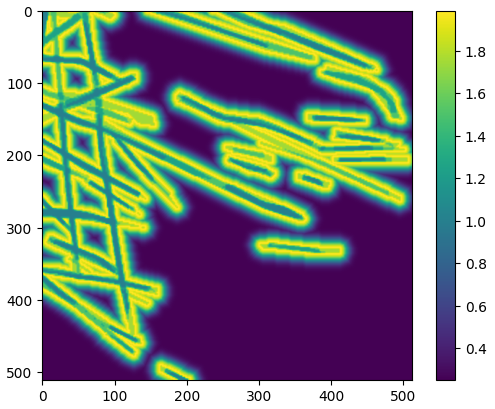\n\n### Optimization:\n\nAdamW, lr schedule: 1 epoch warmup from 2e-4 to 5e-4, CosineAnnealing till the end.\nAll final models were trained for 50 or 64 epochs with pytorch-lightning using bf16 mixed precision.\n\n### Final submission:\nI didn't have much time to train models for building a proper ensemble at the end of the competition, so I had to improvise and include most successful models trained during earlier experiments (which checkpoints are also not lost), which means that the final mix is a bit awkward and all \"survived\" models were trained on the default train/val split (no checkpoints trained on n-fold CV splits):\n\n| weight* | encoder | loss | augs | validation folder only | LB (private) |\n| --- | --- | --- | --- | --- | --- |\n| 0.45 | efficientnet-b7 (smp) | BCE** | Rot90 + Flip + ShiftScaleRotate |0.70030|0.70755|\n| 0.27 | efficientnet-b7 (smp) | 0.98 BCE + 0.02 DICE | Rot90 + Flip + ShiftScaleRotate |0.69794|-|\n| 0.12 | efficientnet-b7 (smp) | BCE** | Rot90 + Flip |0.69524|0.69823|\n| 0.08 | tf_efficientnet_b7 (timm) | BCE** | Rot90 + Flip + ShiftScaleRotate |0.67948|0.67705|\n| 0.08 | tf_efficientnet_b8 (timm) | BCE** | Rot90 + Flip + ShiftScaleRotate |0.68611|0.69415|\n| | **ensemble** | | |**0.70749**|**0.71337**|\n\nAll threshold were tuned on validation folder in logits space rather than in probability space, weighted sum of predictions was also calculated in logits space before transforming to probabilities.\n\n- * Tuned manually on validation folder;\n- ** All these experiments have slightly different pixel weighting parameters in BCE loss.", "2384097": "Congratulations, I wish I had poked around at more channels a bit more. Any hypothesis on why the boost on the private leaderboard?", "2856336": "Congratulations and thanks for sharing, it is a very impressive result, we are particularly attracted by the simplicity of this method, I am wondering if you could kindly send me the source code and the necessary information about it." } }