
First of all, I would like to thank all the organizers of this great contest for all their work and effort.
\nI would also like to thank all participants who shared their ideas and code, especially the gold medal winners of last year's contest.
I didn't do anything special here. I followed the standard calibration notebook and changed the binning value to 4 for AIRS and 48 for FGS.
\nThe technique here is copied from last year's 1st place solution. The curve is smoothed, then, using the points of least and largest derivative value, estimates of the drop transit and rise times are found. These are only initial estimates that will later be refined.
\nTo get the exact times where the transit drop begins and ends, we cut the signal to include only values from the signal's beginning until the initial estimate + a constant value. Then we find 4 values, a, b, t1, and t2, such that the RMSE between the signal and the following function is minimized.
\n
where t1 < t2 and a > b. The desired values are t1 and t2. Those are the exact times the transit drop phase begins and ends, respectively. The exact times for the transit rise start and end are calculated similarly and are called t3 and t4.
\nThis part was hugely inspired by last year's 6th place solution and Vitaly Kudelya's Notebook. For each wavelength, 7 transit depth values were extracted. The values were extracted in the following manner.
\nFirst, for each planet, divide wavelengths into separate groups where neighboring wavelengths go to the same group. Wavelengths in the same group are averaged together (cross-wavelengths) to create a white curve per group.
\nThen, the transit phases are detected in the manner discussed earlier.
\nNext, we calculate the value s that minimizes the MAE of np.concatenate([signal[:t1], signal[t2:t3] * (s + 1.0), signal[t4:]]). Stated more informally, we find the value such that when multiplied by the in-transit section it nearly equals the out-of-transit section, and we subtract 1 from that number. These values are extremely close to the target value; thus, they are great features for the model.
Finally, we give each wavelength in the group that s-value.
\nThis is made 7 times, each time using a different number of groups. The used values are 1, 2, 4, 8, 16, 32, and 64.
\nNow we have 7 values for each of the 283 wavelengths.
\nWe have features of shape (num_planets, 7, num_wavelengths). We also extract the Rs and i values of each planet, making a tensor of shape (num_planets, 2). Both tensors are passed to a neural network.
\nSince important information can be extracted from neighboring wavelengths, the features tensor is passed through three 1D-CNN layers with increasing kernel size and ReLU between them. The last CNN has an out_channels value of 1. Its output is squeezed to form a tensor of shape (batch_size, num_wavelengths).
\nThe CNN output is concatenated on the second axis with the star information (Rs and i). The data is then passed into three ResNet blocks. The final output has shape (batch_size, num_wavelengths).
\nThe model is trained with the Adam optimizer and MSE loss for 300 epochs.
\nThe final output is the predicted spectrum.
\nPredicting the sigma value proved challenging, and different methods significantly impacted the public LB score (with overconfident methods yielding a score of 0.0 on the LB). Two solutions showed great results.
\nThe first was calculating the standard deviation of the predicted spectrum for each planet. Then, the values are scaled to a new mean. The other was calculating for each planet the variance of its white curve, and also scaling it to a new mean.
\nPerforming linear regression on these two features and the mean of the predicted spectrum showed great improvement.
\nYou can access the winning notebook here. There is also a repo for this project containing the code used in the winning submission and other experiments. It also contains more information on the code and how to use it in Kaggle submissions. You can access it here.
\nThere are so many people whose work helped me build mine. To keep this write-up short, I wrote the references section in the GitHub repo for this project. You can find the references section here.
", "messages": [ { "id": 3295150, "postDate": "2025-09-27T19:43:13.930Z", "content": "First of all, I would like to thank all the organizers of this great contest for all their work and effort.
\nI would also like to thank all participants who shared their ideas and code, especially the gold medal winners of last year's contest.
I didn't do anything special here. I followed the standard calibration notebook and changed the binning value to 4 for AIRS and 48 for FGS.
\nThe technique here is copied from last year's 1st place solution. The curve is smoothed, then, using the points of least and largest derivative value, estimates of the drop transit and rise times are found. These are only initial estimates that will later be refined.
\nTo get the exact times where the transit drop begins and ends, we cut the signal to include only values from the signal's beginning until the initial estimate + a constant value. Then we find 4 values, a, b, t1, and t2, such that the RMSE between the signal and the following function is minimized.
\n
where t1 < t2 and a > b. The desired values are t1 and t2. Those are the exact times the transit drop phase begins and ends, respectively. The exact times for the transit rise start and end are calculated similarly and are called t3 and t4.
\nThis part was hugely inspired by last year's 6th place solution and Vitaly Kudelya's Notebook. For each wavelength, 7 transit depth values were extracted. The values were extracted in the following manner.
\nFirst, for each planet, divide wavelengths into separate groups where neighboring wavelengths go to the same group. Wavelengths in the same group are averaged together (cross-wavelengths) to create a white curve per group.
\nThen, the transit phases are detected in the manner discussed earlier.
\nNext, we calculate the value s that minimizes the MAE of np.concatenate([signal[:t1], signal[t2:t3] * (s + 1.0), signal[t4:]]). Stated more informally, we find the value such that when multiplied by the in-transit section it nearly equals the out-of-transit section, and we subtract 1 from that number. These values are extremely close to the target value; thus, they are great features for the model.
Finally, we give each wavelength in the group that s-value.
\nThis is made 7 times, each time using a different number of groups. The used values are 1, 2, 4, 8, 16, 32, and 64.
\nNow we have 7 values for each of the 283 wavelengths.
\nWe have features of shape (num_planets, 7, num_wavelengths). We also extract the Rs and i values of each planet, making a tensor of shape (num_planets, 2). Both tensors are passed to a neural network.
\nSince important information can be extracted from neighboring wavelengths, the features tensor is passed through three 1D-CNN layers with increasing kernel size and ReLU between them. The last CNN has an out_channels value of 1. Its output is squeezed to form a tensor of shape (batch_size, num_wavelengths).
\nThe CNN output is concatenated on the second axis with the star information (Rs and i). The data is then passed into three ResNet blocks. The final output has shape (batch_size, num_wavelengths).
\nThe model is trained with the Adam optimizer and MSE loss for 300 epochs.
\nThe final output is the predicted spectrum.
\nPredicting the sigma value proved challenging, and different methods significantly impacted the public LB score (with overconfident methods yielding a score of 0.0 on the LB). Two solutions showed great results.
\nThe first was calculating the standard deviation of the predicted spectrum for each planet. Then, the values are scaled to a new mean. The other was calculating for each planet the variance of its white curve, and also scaling it to a new mean.
\nPerforming linear regression on these two features and the mean of the predicted spectrum showed great improvement.
\nYou can access the winning notebook here. There is also a repo for this project containing the code used in the winning submission and other experiments. It also contains more information on the code and how to use it in Kaggle submissions. You can access it here.
\nThere are so many people whose work helped me build mine. To keep this write-up short, I wrote the references section in the GitHub repo for this project. You can find the references section here.
", "rawMarkdown": "First of all, I would like to thank all the organizers of this great contest for all their work and effort.\nI would also like to thank all participants who shared their ideas and code, especially the gold medal winners of last year's contest.\n\n# The 48th Place Solution\n\n## Data Calibration\n\nI didn't do anything special here. I followed the standard calibration notebook and changed the binning value to 4 for AIRS and 48 for FGS.\n\n## Transit Detection\n\nThe technique here is copied from [last year's 1st place solution](https://www.kaggle.com/competitions/ariel-data-challenge-2024/writeups/c-number-daiwakun-1st-place-solution). The curve is smoothed, then, using the points of least and largest derivative value, estimates of the drop transit and rise times are found. These are only initial estimates that will later be refined.\n\nTo get the exact times where the transit drop begins and ends, we cut the signal to include only values from the signal's beginning until the initial estimate + a constant value. Then we find 4 values, *a*, *b*, *t1*, and *t2*, such that the RMSE between the signal and the following function is minimized.\n\n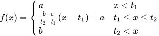\n\nwhere *t1 < t2* and *a > b*. The desired values are *t1* and *t2*. Those are the exact times the transit drop phase begins and ends, respectively. The exact times for the transit rise start and end are calculated similarly and are called *t3* and *t4*.\n\n## Feature Extraction\n\nThis part was hugely inspired by last year's [6th place solution](https://www.kaggle.com/competitions/ariel-data-challenge-2024/writeups/through-the-thorns-to-the-star-6th-place-solution) and [Vitaly Kudelya's Notebook](https://www.kaggle.com/code/vitalykudelya/neurips-non-ml-transit-curve-fitting). For each wavelength, 7 transit depth values were extracted. The values were extracted in the following manner.\n\nFirst, for each planet, divide wavelengths into separate groups where neighboring wavelengths go to the same group. Wavelengths in the same group are averaged together (cross-wavelengths) to create a white curve per group.\n\nThen, the transit phases are detected in the manner discussed earlier.\n\nNext, we calculate the value *s* that minimizes the MAE of `np.concatenate([signal[:t1], signal[t2:t3] * (s + 1.0), signal[t4:]])`. Stated more informally, we find the value such that when multiplied by the in-transit section it nearly equals the out-of-transit section, and we subtract 1 from that number. These values are extremely close to the target value; thus, they are great features for the model.\n\nFinally, we give each wavelength in the group that s-value.\n\nThis is made 7 times, each time using a different number of groups. The used values are 1, 2, 4, 8, 16, 32, and 64.\n\nNow we have 7 values for each of the 283 wavelengths.\n\n## Spectrum Prediction\n\nWe have features of shape (num_planets, 7, num_wavelengths). We also extract the Rs and i values of each planet, making a tensor of shape (num_planets, 2). Both tensors are passed to a neural network.\n\nSince important information can be extracted from neighboring wavelengths, the features tensor is passed through three 1D-CNN layers with increasing kernel size and ReLU between them. The last CNN has an out_channels value of 1. Its output is squeezed to form a tensor of shape (batch_size, num_wavelengths).\n\nThe CNN output is concatenated on the second axis with the star information (Rs and i). The data is then passed into three ResNet blocks. The final output has shape (batch_size, num_wavelengths).\n\nThe model is trained with the Adam optimizer and MSE loss for 300 epochs.\n\nThe final output is the predicted spectrum.\n\n## Sigma Prediction\n\nPredicting the sigma value proved challenging, and different methods significantly impacted the public LB score (with overconfident methods yielding a score of 0.0 on the LB). Two solutions showed great results.\n\nThe first was calculating the standard deviation of the predicted spectrum for each planet. Then, the values are scaled to a new mean. The other was calculating for each planet the variance of its white curve, and also scaling it to a new mean.\n\nPerforming linear regression on these two features and the mean of the predicted spectrum showed great improvement.\n\n## The Code\n\nYou can access the winning notebook [here](https://www.kaggle.com/code/ibrahimhabibeg/lr-sigma-with-nn). There is also a repo for this project containing the code used in the winning submission and other experiments. It also contains more information on the code and how to use it in Kaggle submissions. You can access it [here](https://github.com/ibrahimhabibeg/ariel-2025).\n\n## References and Acknowledgments\n\nThere are so many people whose work helped me build mine. To keep this write-up short, I wrote the references section in the GitHub repo for this project. You can find the references section [here](https://github.com/ibrahimhabibeg/ariel-2025?tab=readme-ov-file#refrences).", "votes": 2 } ], "comments": [], "raw_markdown_by_id": { "3295150": "First of all, I would like to thank all the organizers of this great contest for all their work and effort.\nI would also like to thank all participants who shared their ideas and code, especially the gold medal winners of last year's contest.\n\n# The 48th Place Solution\n\n## Data Calibration\n\nI didn't do anything special here. I followed the standard calibration notebook and changed the binning value to 4 for AIRS and 48 for FGS.\n\n## Transit Detection\n\nThe technique here is copied from [last year's 1st place solution](https://www.kaggle.com/competitions/ariel-data-challenge-2024/writeups/c-number-daiwakun-1st-place-solution). The curve is smoothed, then, using the points of least and largest derivative value, estimates of the drop transit and rise times are found. These are only initial estimates that will later be refined.\n\nTo get the exact times where the transit drop begins and ends, we cut the signal to include only values from the signal's beginning until the initial estimate + a constant value. Then we find 4 values, *a*, *b*, *t1*, and *t2*, such that the RMSE between the signal and the following function is minimized.\n\n\n\nwhere *t1 < t2* and *a > b*. The desired values are *t1* and *t2*. Those are the exact times the transit drop phase begins and ends, respectively. The exact times for the transit rise start and end are calculated similarly and are called *t3* and *t4*.\n\n## Feature Extraction\n\nThis part was hugely inspired by last year's [6th place solution](https://www.kaggle.com/competitions/ariel-data-challenge-2024/writeups/through-the-thorns-to-the-star-6th-place-solution) and [Vitaly Kudelya's Notebook](https://www.kaggle.com/code/vitalykudelya/neurips-non-ml-transit-curve-fitting). For each wavelength, 7 transit depth values were extracted. The values were extracted in the following manner.\n\nFirst, for each planet, divide wavelengths into separate groups where neighboring wavelengths go to the same group. Wavelengths in the same group are averaged together (cross-wavelengths) to create a white curve per group.\n\nThen, the transit phases are detected in the manner discussed earlier.\n\nNext, we calculate the value *s* that minimizes the MAE of `np.concatenate([signal[:t1], signal[t2:t3] * (s + 1.0), signal[t4:]])`. Stated more informally, we find the value such that when multiplied by the in-transit section it nearly equals the out-of-transit section, and we subtract 1 from that number. These values are extremely close to the target value; thus, they are great features for the model.\n\nFinally, we give each wavelength in the group that s-value.\n\nThis is made 7 times, each time using a different number of groups. The used values are 1, 2, 4, 8, 16, 32, and 64.\n\nNow we have 7 values for each of the 283 wavelengths.\n\n## Spectrum Prediction\n\nWe have features of shape (num_planets, 7, num_wavelengths). We also extract the Rs and i values of each planet, making a tensor of shape (num_planets, 2). Both tensors are passed to a neural network.\n\nSince important information can be extracted from neighboring wavelengths, the features tensor is passed through three 1D-CNN layers with increasing kernel size and ReLU between them. The last CNN has an out_channels value of 1. Its output is squeezed to form a tensor of shape (batch_size, num_wavelengths).\n\nThe CNN output is concatenated on the second axis with the star information (Rs and i). The data is then passed into three ResNet blocks. The final output has shape (batch_size, num_wavelengths).\n\nThe model is trained with the Adam optimizer and MSE loss for 300 epochs.\n\nThe final output is the predicted spectrum.\n\n## Sigma Prediction\n\nPredicting the sigma value proved challenging, and different methods significantly impacted the public LB score (with overconfident methods yielding a score of 0.0 on the LB). Two solutions showed great results.\n\nThe first was calculating the standard deviation of the predicted spectrum for each planet. Then, the values are scaled to a new mean. The other was calculating for each planet the variance of its white curve, and also scaling it to a new mean.\n\nPerforming linear regression on these two features and the mean of the predicted spectrum showed great improvement.\n\n## The Code\n\nYou can access the winning notebook [here](https://www.kaggle.com/code/ibrahimhabibeg/lr-sigma-with-nn). There is also a repo for this project containing the code used in the winning submission and other experiments. It also contains more information on the code and how to use it in Kaggle submissions. You can access it [here](https://github.com/ibrahimhabibeg/ariel-2025).\n\n## References and Acknowledgments\n\nThere are so many people whose work helped me build mine. To keep this write-up short, I wrote the references section in the GitHub repo for this project. You can find the references section [here](https://github.com/ibrahimhabibeg/ariel-2025?tab=readme-ov-file#refrences)." } }